Hello everyone,
I am currently working on an energy system model using OEMOF and facing the challenge of implementing a cost function for a flexible electricity price as well as integrating a solar storage system. Specifically, I aim to calculate the total cost of electricity over a certain period and examine the influence of a flexible electricity price from the supplier.
My objectives are:
- Implementing a cost function that accounts for the flexible electricity price.
- Comparing the total costs with and without solar storage over the same period.
- Analyzing the impact of a flexible electricity price from the supplier on the total costs.
I have already started developing the code but am stuck at some points. Here is a snippet of my current code:
###########################################################################
# imports
###########################################################################
import pandas as pd
import matplotlib.pyplot as plt
import base64
from io import BytesIO
import logging
import os
import pprint as pp
import warnings
from datetime import datetime
import pandas as pd
import matplotlib.pyplot as plt
import pandas as pd
from oemof.tools import logger
import oemof.solph as solph
import matplotlib.pyplot as plt
from oemof.solph import flows
from oemof.solph import EnergySystem
from oemof.solph import Model
from oemof.solph import buses
from oemof.solph import components as cmp
from oemof.solph import create_time_index
from oemof.solph import Flow
from oemof.solph import helpers
from oemof.solph import processing
from oemof.solph import views
import numpy as np
from oemof.solph import constraints
def main():
# *************************************************************************
# ********** PART 1 - Define and optimise the energy system ***************
# *************************************************************************
# Read data file
verbrauchsdaten_mit_pv_file = os.path.join(os.getcwd(), 'verbrauchsdaten_mit_pv.csv')
supplier_cost_file = os.path.join(os.getcwd(), 'Day_Night_price_Supplier_.csv')
verbrauchsdaten_mit_pv_data = pd.read_csv(verbrauchsdaten_mit_pv_file)
supplier_cost_data = pd.read_csv(supplier_cost_file)
solver = "cbc" # 'glpk', 'gurobi',....
debug = False # Set number_of_timesteps to 3 to get a readable lp-file.
solver_verbose = False # show/hide solver output
# initiate the logger (see the API docs for more information)
logger.define_logging(
logfile="oemof_example.log",
screen_level=logging.INFO,
file_level=logging.INFO,
)
date_time_index = pd.date_range('1/1/2024 00:00:00', periods=48, freq='30min')
# create the energysystem and assign the time index
energysystem = EnergySystem(
timeindex=date_time_index, infer_last_interval=False
)
##########################################################################
# Create oemof objects
##########################################################################
logging.info("Create oemof objects")
# The bus objects were assigned to variables which makes it easier to
# connect components to these buses (see below).
# create electricity bus
bel = buses.Bus(label="electricity")
# adding the buses to the energy system
energysystem.add(bel)
# create excess component for the electricity bus to allow overproduction
energysystem.add(cmp.Sink(label="excess_bel", inputs={bel: flows.Flow()}))
energysystem.add(
cmp.Source(
label="supplier",
outputs={
bel: flows.Flow(
nominal_value=1000,
variable_costs=supplier_cost_data["costs"],
custom_attributes={"emission_factor": 0.20},
)
},
)
)
# create fixed source object representing pv power plants
energysystem.add(
cmp.Source(
label="pv",
outputs={bel: flows.Flow(fix=verbrauchsdaten_mit_pv_data["pv"], nominal_value=1000)},
)
)
# create simple sink object representing the electrical demand 1
energysystem.add(
cmp.Sink(
label="consumer1",
inputs={bel: flows.Flow(fix=verbrauchsdaten_mit_pv_data["consumer1"], nominal_value=1, custom_attributes={"emission_factor": 0.60},)},
)
)
# create simple sink object representing the electrical demand 2
energysystem.add(
cmp.Sink(
label="consumer2",
inputs={bel: flows.Flow(fix=verbrauchsdaten_mit_pv_data["consumer2"], nominal_value=1, custom_attributes={"emission_factor": 0.30},)}
)
)
# create storage object representing a battery
storage = cmp.GenericStorage(
nominal_storage_capacity=25000,
label="storage",
inputs={bel: flows.Flow(nominal_value=25000 / 6)},
outputs={
bel: flows.Flow(nominal_value=25000 / 6, variable_costs=0.001)
},
loss_rate=0.00,
initial_storage_level=None,
inflow_conversion_factor=1,
outflow_conversion_factor=0.8,
)
energysystem.add(storage)
##########################################################################
# Optimise the energy system and plot the results
##########################################################################
logging.info("Optimise the energy system")
# initialise the operational model
model = Model(energysystem)
# This is for debugging only. It is not(!) necessary to solve the problem
# and should be set to False to save time and disc space in normal use. For
# debugging the timesteps should be set to 3, to increase the readability
# of the lp-file.
if debug:
filename = os.path.join(
helpers.extend_basic_path("lp_files"), "basic_example.lp"
)
logging.info("Store lp-file in {0}.".format(filename))
model.write(filename, io_options={"symbolic_solver_labels": False})
# if tee_switch is true solver messages will be displayed
logging.info("Solve the optimization problem")
model.solve(solver=solver, solve_kwargs={"tee": solver_verbose})
logging.info("Store the energy system with the results.")
# The processing module of the outputlib can be used to extract the results
# from the model transfer them into a homogeneous structured dictionary.
# add results to the energy system to make it possible to store them.
energysystem.results["main"] = processing.results(model)
energysystem.results["meta"] = processing.meta_results(model)
# The default path is the '.oemof' folder in your $HOME directory.
# The default filename is 'es_dump.oemof'.
# You can omit the attributes (as None is the default value) for testing
# cases. You should use unique names/folders for valuable results to avoid
# overwriting.
# store energy system with results
energysystem.dump(dpath=None, filename=None)
# *************************************************************************
# ********** PART 2 - Processing the results ******************************
# *************************************************************************
logging.info("**** The script can be divided into two parts here.")
logging.info("Restore the energy system and the results.")
energysystem = EnergySystem()
energysystem.restore(dpath=None, filename=None)
# define an alias for shorter calls below (optional)
results = energysystem.results["main"]
storage = energysystem.groups["storage"]
# print a time slice of the state of charge
print("")
print("********* State of Charge (slice) *********")
print(
results[(storage, None)]["sequences"][
datetime(2024, 1, 1, 0, 0, 0) : datetime(2024, 1, 8, 0, 0, 0)
]
)
print("")
# get all variables of a specific component/bus
custom_storage = views.node(results, "storage")
electricity_bus = views.node(results, "electricity")
# plot the time series (sequences) of a specific component/bus
fig, ax = plt.subplots(figsize=(10, 5))
custom_storage["sequences"].plot(
ax=ax, kind="line", drawstyle="steps-post"
)
plt.legend(
loc="upper center",
prop={"size": 8},
bbox_to_anchor=(0.5, 1.25),
ncol=2,
)
fig.subplots_adjust(top=0.8)
plt.show()
fig, ax = plt.subplots(figsize=(10, 5))
electricity_bus["sequences"].plot(
ax=ax, kind="line", drawstyle="steps-post"
)
plt.legend(
loc="upper center", prop={"size": 8}, bbox_to_anchor=(0.5, 1.3), ncol=2
)
fig.subplots_adjust(top=0.8)
plt.show()
# Convert the flow results to DataFrames
df_custom_storage = pd.DataFrame(custom_storage["sequences"])
df_electricity_bus = pd.DataFrame(electricity_bus["sequences"])
# Save the DataFrames to CSV files
df_custom_storage.to_csv("custom_storage_flows.csv")
df_electricity_bus.to_csv("electricity_bus_flows.csv")
# print the solver results
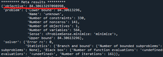
print("********* Meta results *********")
pp.pprint(energysystem.results["meta"])
print("")
# print the sums of the flows around the electricity bus
print("********* Main results *********")
print(electricity_bus["sequences"].sum(axis=0))
# Ergebnisse in csv-Speichern
# Metaergebnisse in DataFrame konvertieren
meta_results = energysystem.results["meta"]
df_meta = pd.DataFrame(meta_results.items(), columns=["Parameter", "Value"])
# CSV-Datei für Metaergebnisse speichern
df_meta.to_csv("meta_results.csv", index=False)
# Hauptergebnisse in DataFrame konvertieren
main_results = electricity_bus["sequences"].sum(axis=0)
df_main = pd.DataFrame({"Time": main_results.index, "Sum of Flows": main_results.values})
# CSV-Datei für Hauptergebnisse speichern
df_main.to_csv("main_results.csv", index=False)
if __name__ == "__main__":
main()
I would greatly appreciate any help, particularly with implementing the cost function and integrating the solar storage system. If anyone has experience with similar issues or suggestions for solving these tasks, I would appreciate any feedback!
Thank you in advance for your assistance.
Best regards,
Armend
CSV.zip (3.0 KB)