We are looking for good modelling patterns in oemof for two heat‑pump use cases that involve both heating and cooling:
Case 1: Heat pump for either heating OR cooling (e.g. single-family-house)
-
Winter: ground‑source HP provides heating.
-
Summer: the same ground‑source HP or a heat exchanger provides cooling.
-
At each timestep the unit should be either in heating mode or in cooling mode, with different COP for both modes.
How can this “either–or” behaviour best be implemented in oemof? Is there a standard way (e.g. with additional constraints, or binaries via oemof.solph) to prevent simultaneous heat and cold production from the same investment?
Case 2: Heat pump for heating AND/OR cooling (e.g. industry, hospital)
-
Winter: ground‑source HP supplies heat.
-
With simultaneous heat and cold demand: HP can upgrade return temperature from the cooling system return. Heat pump can also use a share of each “heat” source!
-
Summer: ground‑source HP or heat exchanger provides cooling.
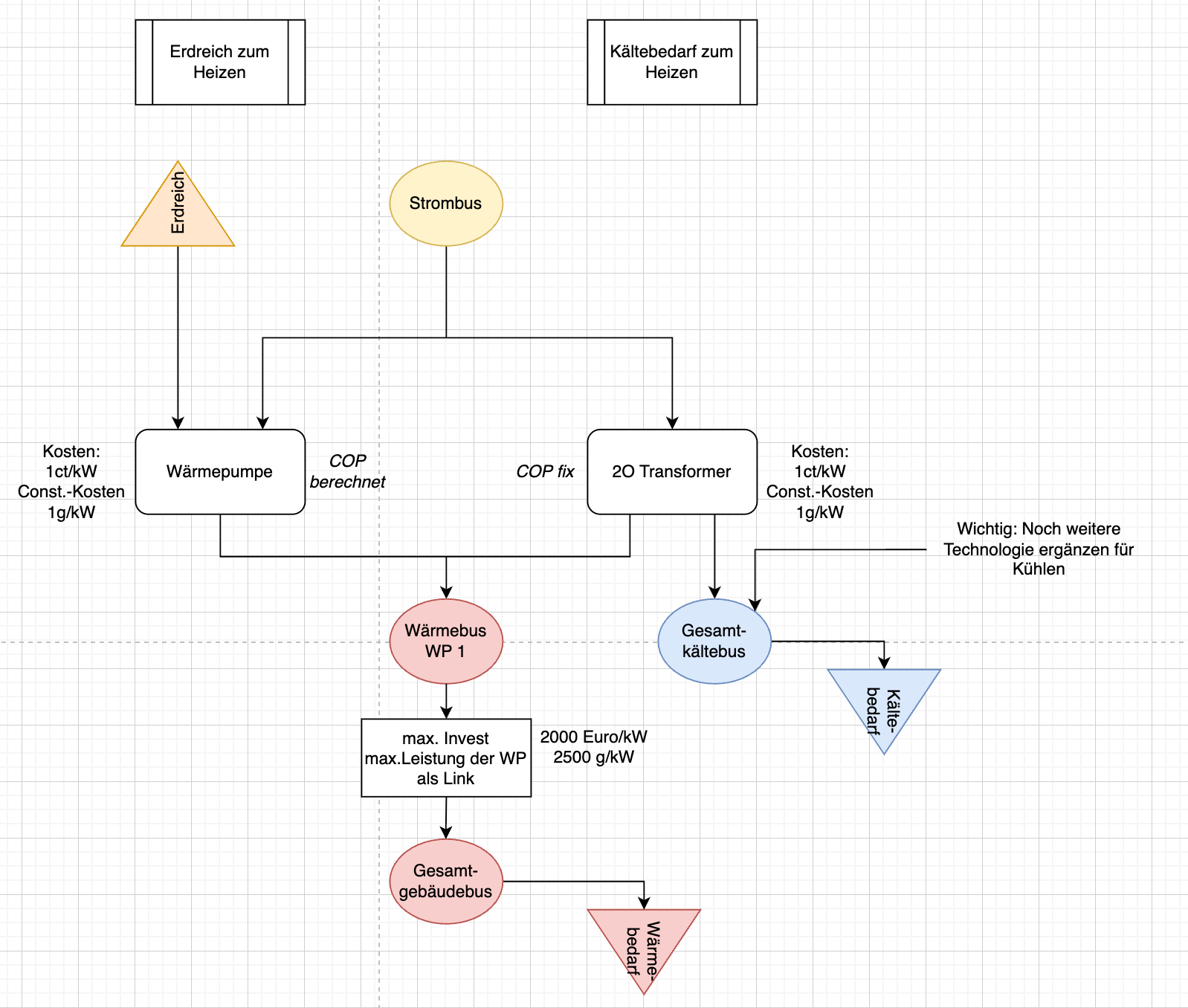
Our current idea is to place the investment on the Link and connect the different low‑temperature sources (ground, return) to it. This idea is sketched in the attached figure (in German). This approach feels like a workaround, and we are not sure whether there is a more transparent or standard way to implement such a multi‑source HP in oemof. Moreover, the “either–or” logic from Case 1 (no simultaneous heating and cooling from the same HP) also appears here and we have not found a solution yet.
Summarized Questions:
-
Recommended way in oemof.solph to model a HP that can either heat or cool in one timestep?
-
Modelling pattern for a multi‑source HP (ground + return) with a single compressor investment?
-
Any existing examples or publications that deal with similar heating/cooling HP use cases?
Hi @Franzi041!
I’d tend to model the cooling demand as a waste heat sources. As different COPs for heating and cooling are just the expression of the conservation of energy (Inflow + Electricity = Outflow <=> COP_cooling * Electricity + Electricity = COP_heating * Electricity ), that can simplifies the model by quite a lot.
Furthermore, while it is technically possible (se limit_active_flow_count in the docs), I strongly recommend not to code either/or logics into the model. It can turn your optimisation problem into a combinatorial one and make your computational time explode. (That is because of the fundamental nature of such constraints, we can’t do anything about that.) Instead, I’d add a common “resource” bus as described also in [2012.12664] Simultaneous optimisation of temperature and energy in linear energy system models .
In fact, the heat pump use case is my favourite one to play around with when developing MTRESS, which also serves as our (DLR) playground for fancy new features related to oemof.solph. We are currently aligning this with current solph, so that it will be more interoperable. A (directly usable) heat pump model is hopefully done by the end of the next week. (Just having a look might be overwhelming because we are very generic and don’t just implement ne model. Also, we currently prototype without caring too much about the documentation. But feel free to have a look.)
thanks a lot for your explanations so far – they already helped me a lot to understand the general idea.
I’m still struggling a bit with the concrete implementation, though. Would you maybe have a small oemof.solph example for my Case 1 (single reversible heat pump for either heating or cooling), using:
-
a common “resource” bus for the heat pump capacity, and
-
the cooling demand modelled as a waste‑heat source, as you suggested?
I think I understand the general idea from your paper and the description with the status variables, but I’m not yet sure how to translate this into a concrete solph mode
Hi @Franzi041,
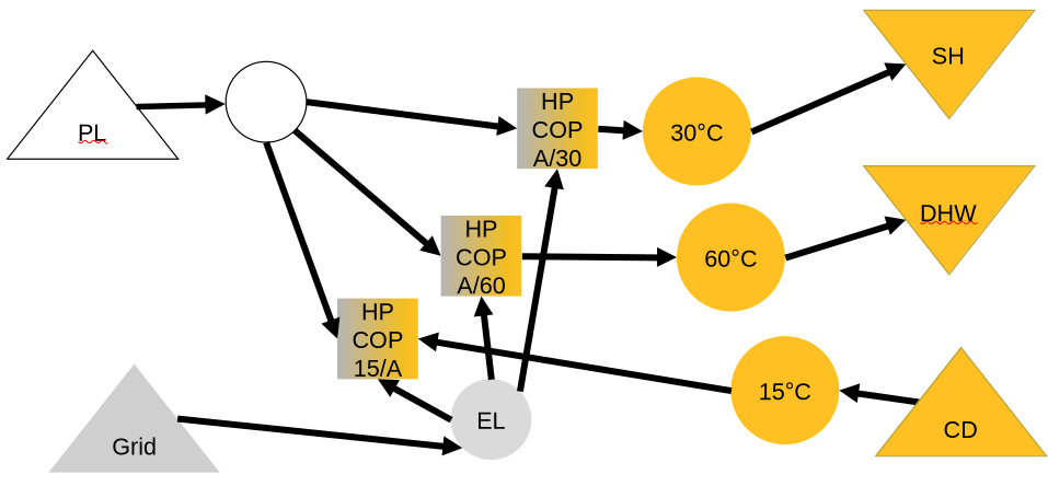
unfortunately, the ready to use heat pump is not done, yet. However, I am preparing a lecture at the moment and here is a sketch, I prepared for it:
The legend is as follows:
- Box: Converter
- Circle: Bus
- Pyramid triangle: Source
- Triangle pointing down: Sink
The heat sector is coloured yellow, electricity is grey. You see that the converters connect the two. The special thing is the “source” PL, which is for “Part Load”. Its outflow is limited to 1, so e.g. you can have 50 % of the load for heating and 50 % for cooling. (It is not strict one at a time, but as good as it gets linearly.)
I hope this makes the idea pretty clear. (If not, I appreciate feedback, in particular as I can need it for the lecture.)
The heating, ventilation, and air conditioning (HVAC) module described in my PhD report and coded in C++ might be of interest, see specifically:
- §7.11: HVAC air conditioning model
- Appendix 1: Plank refrigeration model (with R‑134a characterization)
That report is here:
- Morrison, Robbie (January 2026). High‑resolution simulation and analysis of complex energy systems — PhD thesis. Berlin, Germany: Technical University of Berlin. doi:10.14279/depositonce-24931. Release 09.
Note however (page 76):
The HVAC component consists of two parts. Air chilling is undertaken using an electrically driven vapor-compression refrigerator charged with R-134a, a common haloalkane refrigerant. Air heating employs simple resistance heating.
Not quite what was requested but surely no trouble to run the AC unit in reverse as a heat pump.
The associated code (.h are the C++ header files as linked below, .cc are the C++ implementation files which you can find in the same subdirectory):
The software license is GPL‑3.0‑or‑later.
All lead‑up work is cited, should you wish to dig down further. For related background on this site, search for “Plank”. PM me if you want a copy of Plank (1940). HTH, R. Pinging @Franzi041.
▢
While on the topic of refrigerants and such, this podcast (01:05:50) might help (RMI was previously the Rocky Mountain Institute):
The global warming potential (GWP) of R‑134a is 1430 over a 100-year timeframe, so perhaps try something else?
▢
Thank you! The idea in general is clear.
My question is: in the oemof model, the pl source is treated as a real energy flow (with units, e.g. kW) or as a dimensionless control signal (0…1, representing “part‑load share”)?
If its outflow is capped at 1, but the connected converters also have physical energy inputs (electricity, heat), how exactly is this “1” combined with those flows in the equations? Is PL part of the energy balance, or only used to weight/limit the operation of the different converters (heating vs cooling)?
Do I need to use an equate flow (oemof.solph.constraints - v0.6.4)?
Also where do I consider the investment costs of the components?
My question is: in the oemof model, the pl source is treated as a real energy flow (with units, e.g. kW) or as a dimensionless control signal (0…1, representing “part‑load share”)?
If its outflow is capped at 1, but the connected converters also have physical energy inputs (electricity, heat), how exactly is this “1” combined with those flows in the equations? Is PL part of the energy balance, or only used to weight/limit the operation of the different converters (heating vs cooling)?[/quote]
Technically, it is always a control signal. Whether you make it dimensionless or in units of energy is actually up to you. (It will never be part of the energy balance, though.) As you also give corresponding conversion_factors, both are equivalent: For power, the conversion_factor would be {b_pl: 1} or maybe {b_pl: 0.8} if you want to scale it down for one of the paths. For the control signal you give the nominal outlet power as conversion factor. The beauty of this approach is, that you do not need any additional constraints besides the ones already in the converters.
1) Case A (PL as power, conversion_factor[b_pl] = 1)
If I set the conversion factor for the PL bus to 1, does that mean that the energy flow over this bus – and therefore the PL source – “takes over” the realistic maximal investment capacity and the associated costs and emissions?
In other words: Is the PL flow effectively the installed capacity (or part of it) and should I then attach costs/emissions to the PL source, or should all costs/emissions still only be attached to the real energy inputs (electricity, heat) and the output investment?
2) Case B (PL as pure control signal, conversion_factor[b_pl] = P_nom)
You mention that for a pure control signal, one can use the nominal outlet power as conversion factor, i.e. {b_pl: P_nom}. Is Case B also possible if PnomP_\text{nom}Pnom is only determined during the optimization (via an Investment)?
Since conversion_factors are parameters fixed before solving, I’m unsure how to implement Case B when the installed capacity PnomP_\text{nom}Pnom is not known a priori but is an optimization result. Do you see a recommended way to handle this situation, or would you say Case B only really works when PnomP_\text{nom}Pnom is a given technical design value (not an optimized one)?
Small aside: the forum software uses CommonMark markdown for markup and offers LaTeX‑like syntax for mathematics, as described here: Discourse Math - Plugin - Discourse Meta 
You are right, @Franzi041, if you want to optimise capacities using investment costs for thermal power, this is easier when you have PL as power. Actually, a normalised control signal does not directly work with investments. There are possible workarounds but I would just not do that way, just pick case A.
This model to support the operational planning of district heating systems from one of the Fraunhofer research institutes might offer some clues: https://open.pages.fraunhofer.de/iosb/mrd/terms/explorer/mop.html. It looks very object‑oriented but beyond that, I cannot say very much.
Update: this software is not open‑source.
This Municipal Heat Planning Ontology (MHPO) to support municipal heat planning might also be relevant for some applications: https://github.com/OpenEnergyPlatform/municipal-heat-planning-ontology