Dear community,
i have the problem that i want to model a power plant where the conversations factor is dependent on the produced heat. Is that feasible? And if so, how?
Thanks in advance for your help.
CS
Dear community,
i have the problem that i want to model a power plant where the conversations factor is dependent on the produced heat. Is that feasible? And if so, how?
Thanks in advance for your help.
CS
Hi,
if you have something in mind like a combined cycle extraction turbine you could have a look at the solph-component GenericCHP. It allows you to define an electric power loss through heat extraction (Beta). You will find detailed information here: oemof-solph documentation.
Does that component work for you?
Best,
Jakob
The GenericCHP class leads to a MILP, the ExtractionTurbineCHP is fully linear, but less exact. Both components can vary the fraction of heat and power but not the overall efficiency.
If you want a non linear relation between the efficiency and the output you should take a look at the offset transformer (MILP).
Furthermore, the Piecewise linear transformer is planed for v0.4.1 but you can always help to speed up the development.
My answer here is for a one‑product process but it should be straightforward to generalize to a multi‑product and/or multi‑fuel process. While on preliminaries, an arbitrary characteristic curve can be modeled using piecewise linearization and SOS2 sets, but this will entail a computational cost. The method shown here instead introduces just one binary variable to toggle between operation and shutdown. It is worth giving a reasonably full response because this technique is generally quite useful for energy system models based on linear programming.
The following treatment assumes recursive dynamic (colloquially rolling) optimization. It may need to be simplified for full horizon optimization depending on the information available when the linear problem is fixed and passed to the solver.
The operation of technical assets at light duty is regularly avoided in practice, usually because the off‑design efficiency can be quite low (even though optimization-based unit-commitment can naturally account for this deterioration).
So we let the plant trip at some specified threshold p_\mathrm{lower} as shown in the following diagram. While p_\mathrm{upper} is the current maximum capacity and may depend on the prevailing environmental conditions (such as ambient air temperature) and plant state (thereby allowing ramp up restrictions to be honored, for example) as calculated in a prior step before optimization. And 1/m is the marginal efficiency and necessarily constant in this formulation.
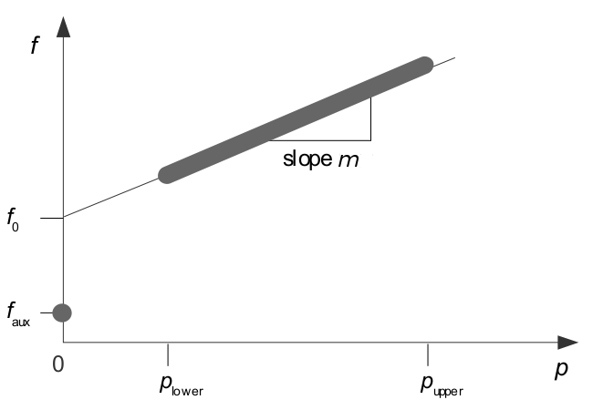
Figure 1: An input/output diagram showing the solution space available for shutdown mode operation. Only the gray regions are admissible.
Assuming, for the moment, that the auxiliary fuel requirement f_\mathrm{aux} is deemed zero, the following equations apply:
where p indicates the product and f indicates the fuel (or more generally, factor input) and subject to:
If the auxiliary fuel requirement is nonzero, meaning circulation pumps and similar should continue to run, then the first equation becomes:
When in run mode, the above equation can be recast as an efficiency:
This form of equation is known as the Michaelis‑Menton relation and is one of several models commonly used in nonlinear regression (Crawley 2007:662).
The parameters m and f_0 can usually be estimated from published empirical data under standard condition, namely \eta (or f) at p_\textrm{lower} and p_\textrm{upper}. If performance curves are available, they should be overplotted to check for discrepancies. Be aware too that performance conventions in Europe and North America may differ.
Under shutdown:
The information in figure 1 can be replotted. Generally speaking, it is the average efficiency that informs unit commitment.
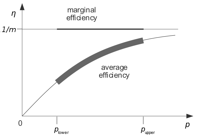
Figure 2: An efficiency diagram showing the same information given earlier.
All the parameters listed can be calculated for each time‑step depending on ambient conditions and plant status. These dependencies need not be linear but they must be explicit.
As noted at the outset, the input/output relationship in figure 1 can be piecewise linear and the method can be extended to cater for multi‑factor and multi‑product technologies.
Finally, a ratio of p_\textrm{lower} to p_\textrm{upper} of about 50% seems to work quite well and is usually defensible in practice too.
Crawley, Michael J (2007). The R book (reprinted with corrections 2009). Chichester, United Kingdom: John Wiley and Sons. ISBN 978-0-470-51024-7.