I am looking for an open-source energy modelling tool for doing a dynamic simulation of a direct solar running drinking water system (without any storage), working with the Flash evaporation process.
Here is a schematic layout of the process:
Due to the variable solar power, the goal of the project is to find out in which partial loads all the components must operate to bring the maximum output of drinking water in a wide range of available power.
In this context, the dynamic simulation should be able to calculate in every new time step the maximum output. If I understand correctly, the steady state simulation could only optimize the system for getting the maximum output for the whole day, instead of every time step. But I am only a beginner in energy modelling, so I am not sure about it.
I already tried to model the system in TESPy, but here a distributor told me that is it not possible to perform dynamic simulations within the package.
Any help is much appreciated.
Many thanks in advance!
I don’t have a comprehensive answer but let me make some points. First, I take it the problem attributes include:
that this is an optimization problem — meaning the system is not fully constrained by the problem definition and at least one decision variable remains open
the goal function is to seek maximum output over the nominated time‑horizon
this is solely an operational problem, component sizing is not part of the research question and therefore not part of the solution space
there are no dedicated flow‑related intertemporal connections between timesteps — covering things like thermal storage, product storage, or demand displacement
indeed, there is no demand timeseries that needs servicing
the environment is fully known at the outset — so influential variables like the solar resource and ambient temperature are predefined as timeseries
for convenience, let’s assume your timesteps are one hour — this is somewhat arbitrary but it makes it easier to think about the problem
Regarding terminology, “dynamic” may describe a fully‑constrained problem or it may describe an optimization problem with at least one decision variable left open and a goal function to guide the outcome. More specifically, recursive dynamic optimization is sometimes used to convey optimization that proceeds from one timestep to the next, resetting the problem as it proceeds. In short, the term “dynamic” can cover many concepts, so it is important to clarify which one you mean.
For maximum output flow‑based optimization of your system, you may need to assume your system’s intensive state and extensive state can can be set sequentially and orthogonally. Moreover the system settles quickly into this new state relative to the time interval in use.
I am not quite sure why you indicated (did I get that right) that overall output is not simply the arithmetic sum of the individual outputs at each timestep —is there some intertemporal effect that I am missing — like thermal inertia, for example? It might be useful to note down the following to fill in the gaps:
the decision variables — not clear to me what these are — also perhaps you can mark some intensive and extensive state variables and also predetermined constants on your diagram?
One hint is that you might need to proxy the control system in place — usually present to maintain some given intensive state under a range of extensive states and environmental conditions. The deeco framework did this for flow‑and‑return‑based heat transfer.
Another hint is to look at analytical methods that predate numerics. One such example is the Plank refrigerant model (Plank 1940) (PM me for a copy) that has been adapted for use in mathematical programs. Of course, no one would use such methods today for pure simulation purposes but they may usefully deployed in this context? An implementation using C++ can be found here. That paper:
Plank, Rudolf (1940). “Zur thermodynamischen Bewertung von Kältemitteln” [On the thermodynamic evaluation of refrigerants] (in German). Zeitschrift für die gesamte Kälte-Industrie. 6: 81–84. Copy in TU Berlin library.
I guess AI‑based methods are on the cards if you can access suitable historical data.
Unless you are lucky enough to find a prior module for flash evaporation, you’ll probably need to be quite innovative in the way you structure your problem relative to your research objectives and data sources.
Thank you for helping to clear up the problem attributes and giving some hints.
In the attributes that you included I can fully agree.
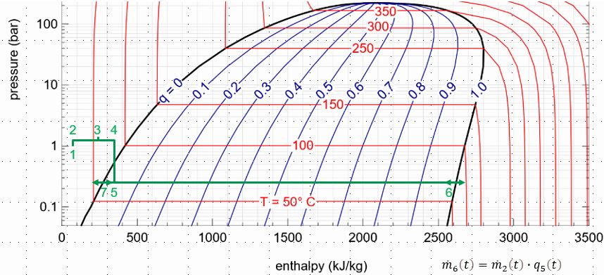
You indicate, I may assume to set the intensive and extensive orthogonally - hence, so they dont interfere with each other. Im unsure if thats possible for the extensive varibale enthalpy? Because isnt the enthalpy very much dependent from the pressure and the temperature?
The thermal inertia is indicated in the diagram by Q_heat exchanger and Q_tank. It probably only has a big impact for the start process in the morning (heat exchanger and tank has to get heated up). If the temperatures do not change significantly, it maybe possible to divide the problem in two parts:
The start process including the thermal inertias.
The ongoing process excluding the thermal inertias.
One decision variable may be the temperature 4. In the literature called the - Top Brine Temperature (TBT). The manufacture Wärtsilä set for the systems a TBT of 80°C.
Fully known is only the state of the seawater in 1. I will mark other constants and state variables later on in the diagram.
Enthalpy is a function of temperature and pressure, of course. For linear programming, the question is can you determine those temperatures and pressures in a first step and then optimize your system flows (under the so‑called minimum‑cost flow problem or MCFP formulatoin) in a second step, relative to your goal function (whether least OPEX, least carbon, or maximum product), without disturbing those earlier temperatures and pressures?
To use an electricity analogy, can you set your target voltage (to say 11 kV) and then later determine your load flows (say in kW) without disturbing that target voltage? In most cases, the answer is yes. For instance, utility scale batteries will drop voltage under load, but there is usually a ton of power electronics, tap‑changing transformers, and so on to compensate.
The enthalpy inventories in these components should not be a problem unless the state orthogonality assumption we’ve been discussing falls down. These are just forms of storage. You can assume good mixing or you can model stratified storage, as appropriate. There is some literature on thermal storage (I have 5 references databased) and several implementations too.
I am not convinced that you need to determine two regimes: start-up and normal operations.
But it may well be that your plant is not amenable to an MCFP formulation? I cannot tell from this distance which assumptions can be supported or which cannot … while noting that MCFP is not the only show in town. This is all the art of modeling of course. Happy hacking!
if I recall correctly we discussed this in a call, or? Since you are asking here, I’ll just add the info for everyone interested:
for this case you could actually use tespy and it would bring all requirements with it :). The startup process (or any other dynamic phenomena of ramping and having fluid flow propagate dynamically through the components) does indeed not work with tespy!
And to note that simulation applications can be useful for characterizing some system of interest by allowing their components to be represented “empirically” in flow optimization frameworks … given that you have some luck on your side!
The mass flow 6 is our desired output, which we want to maximize. For doing that we want to have the biggest possible vapor content (q) in point 5. The vapor content is very much depended on the intensiv states.
I believe that in the system, the set parameters temperature and pressure must be changed for getting the maximum output and with that MCFP formulation does not work anymore. So then TESPy and oemof will not be accurate, or am I wrong?
@MMueller Two small points. First, based on your initial description, your problem formation is probably the maximum flow problem (MFP) rather than the MCFP. The underlying system definition is the same in both cases — so that’s no big deal.
Second, I’ll PM you (later today) with an example using R‑134a data and the Plank refrigerant model mentioned earlier. In this case, the refrigeration process was amenable to a mathematical programming (MP) formulation. The needed R‑134a property values were calculated using RefCalc 2.03, published by the Technical University of Denmark.
To respond to your question in the context of oemof at least, there is noa priori answer. You may be able to shoe‑horn your process into a mathematical program … or you might not. I have an MP model of a CCGT gas turbine that cuts out below 50% duty that matches the empirical operating curve remarkably well. A happy accident I suppose? Other processes may not be so mathematically compliant.
Without getting into the depths of flash evaporation, that’s all I can say. HTH, R
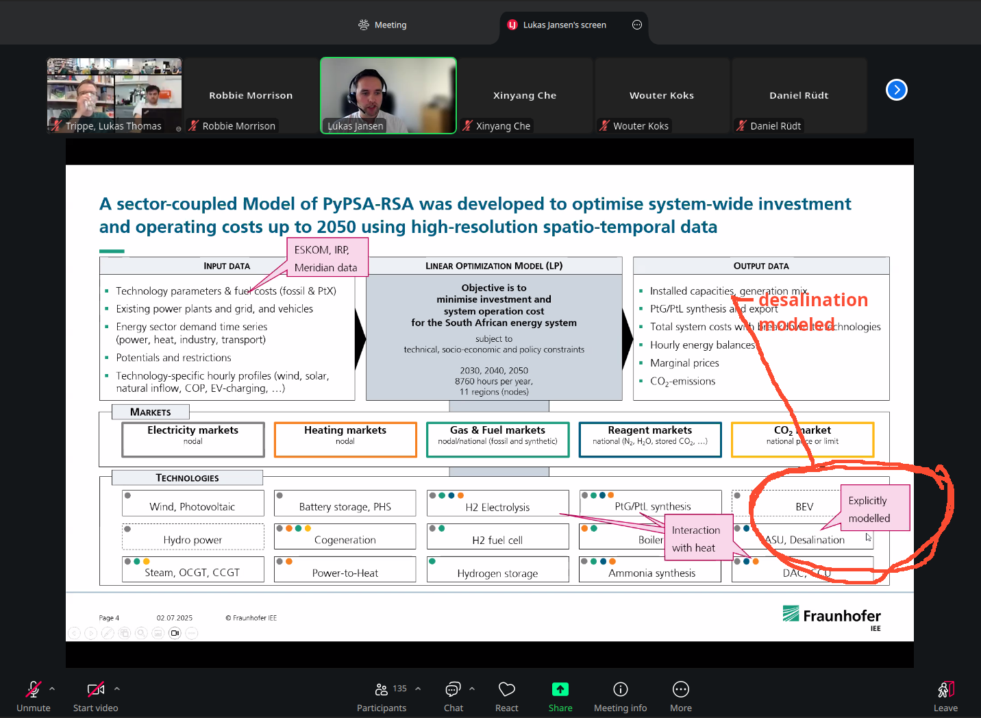
Thank you for thinking of me. I worked with PyPSA before and I think it will not serve my project so well. Or did Lukas Jansen say, the he modelled the desalination separately?
I know, its a far step away from MILP/LP solvers like PyPSA and OEMOF, but had you already looked into Modelica? I haven’t fully understood your main objective (high level model with focus on economic dispatch or more towards detailled physics), but I guess especially when you want to represent the fluid in a realistic way with detailled thermodynamic modeling, it will be very difficult to represent that with decision variables and linear relationships.
The tradeoff, you would need to do the optimization manually (varying your decision variables) or with some external loop using metaheuristic optimizer.
It is also not entirely clear for me, what the characteristics you want to consider (dynamics or stationary operation). tespy works perfectly fine to find the maximum mass flow/vapor content in stationary operation. You can simply call the tespy model with variable inputs for pressure/temperature through scipy or use the pygmo API of tespy.